Heat equation

28 languages

• Article
• Talk

• Read
• Edit
• View history

From Wikipedia, the free encyclopedia

Animated plot of the evolution of the temperature in a square metal plate as predicted by the heat equation. The height and redness indicate the temperature at each point. The initial state has a uniformly hot hoof-shaped region (red) surrounded by uniformly cold region (yellow). As time passes the heat diffuses into the cold region.

In mathematics and physics, the heat equation is a certain partial differential equation. Solutions of the heat equation are sometimes known as caloric functions. The theory of the heat equation was first developed by Joseph Fourier in 1822 for the purpose of modeling how a quantity such as heat diffuses through a given region.

As the prototypical parabolic partial differential equation, the heat equation is among the most widely studied topics in pure mathematics, and its analysis is regarded as fundamental to the broader field of partial differential equations. The heat equation can also be considered on Riemannian manifolds, leading to many geometric applications. Following work of Subbaramiah Minakshisundaram and Åke Pleijel, the heat equation is closely related with spectral geometry. A seminal nonlinear variant of the heat equation was introduced to differential geometry by James Eells and Joseph Sampson in 1964, inspiring the introduction of the Ricci flow by Richard Hamilton in 1982 and culminating in the proof of the Poincaré conjecture by Grigori Perelman in 2003. Certain solutions of the heat equation known as heat kernels provide subtle information about the region on which they are defined, as exemplified through their application to the Atiyah–Singer index theorem.^[1]

The heat equation, along with variants thereof, is also important in many fields of science and applied mathematics. In probability theory, the heat equation is connected with the study of random walks and Brownian motion via the Fokker–Planck equation. The Black–Scholes equation of financial mathematics is a small variant of the heat equation, and the Schrödinger equation of quantum mechanics can be regarded as a heat equation in imaginary time. In image analysis, the heat equation is sometimes used to resolve pixelation and to identify edges. Following Robert Richtmyer and John von Neumann's introduction of "artificial viscosity" methods, solutions of heat equations have been useful in the mathematical formulation of hydrodynamical shocks. Solutions of the heat equation have also been given much attention in the numerical analysis literature, beginning in the 1950s with work of Jim Douglas, D.W. Peaceman, and Henry Rachford Jr.

Statement of the equation[edit]

In mathematics, if given an open subset U of Rⁿ and a subinterval I of R, one says that a function u : U × I → R is a solution of the heat equation if

${\displaystyle \frac{\mathrm{\partial }�}{\mathrm{\partial }�}=\frac{{\mathrm{\partial }}^2�}{\mathrm{\partial }{�}_1^2}+\cdots +\frac{{\mathrm{\partial }}^2�}{\mathrm{\partial }{�}_{�}^2},}$

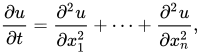
where (x₁, …, x_n, t) denotes a general point of the domain. It is typical to refer to t as "time" and x₁, …, x_n as "spatial variables," even in abstract contexts where these phrases fail to have their intuitive meaning. The collection of spatial variables is often referred to simply as x. For any given value of t, the right-hand side of the equation is the Laplacian of the function u(⋅, t) : U → R. As such, the heat equation is often written more compactly as

${\displaystyle \frac{\mathrm{\partial }�}{\mathrm{\partial }�}=\mathrm{\Delta }�}$.

In physics and engineering contexts, especially in the context of diffusion through a medium, it is more common to fix a Cartesian coordinate system and then to consider the specific case of a function u(x, y, z, t) of three spatial variables (x, y, z) and time variable t. One then says that u is a solution of the heat equation if

${\displaystyle \frac{\mathrm{\partial }�}{\mathrm{\partial }�}=�\left(\frac{{\mathrm{\partial }}^2�}{\mathrm{\partial }{�}^2}+\frac{{\mathrm{\partial }}^2�}{\mathrm{\partial }{�}^2}+\frac{{\mathrm{\partial }}^2�}{\mathrm{\partial }{�}^2}\right)}$

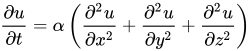
in which α is a positive coefficient called the thermal diffusivity of the medium. In addition to other physical phenomena, this equation describes the flow of heat in a homogeneous and isotropic medium, with u(x, y, z, t) being the temperature at the point (x, y, z) and time t. If the medium is not homogeneous and isotropic, then α would not be a fixed coefficient, and would instead depend on (x, y, z); the equation would also have a slightly different form. In the physics and engineering literature, it is common to use ∇² to denote the Laplacian, rather than ∆.

In mathematics as well as in physics and engineering, it is common to use Newton's notation for time derivatives, so that ${\displaystyle \dot{�}}$ is used to denote ∂u/∂t, so the equation can be written

${\displaystyle \dot{�}=\mathrm{\Delta }�}$.

Note also that the ability to use either ∆ or ∇² to denote the Laplacian, without explicit reference to the spatial variables, is a reflection of the fact that the Laplacian is independent of the choice of coordinate system. In mathematical terms, one would say that the Laplacian is "translationally and rotationally invariant." In fact, it is (loosely speaking) the simplest differential operator which has these symmetries. This can be taken as a significant (and purely mathematical) justification of the use of the Laplacian and of the heat equation in modeling any physical phenomena which are homogeneous and isotropic, of which heat diffusion is a principal example.

The "diffusivity constant" α is often not present in mathematical studies of the heat equation, while its value can be very important in engineering. This is not a major difference, for the following reason. Let u be a function with

${\displaystyle \frac{\mathrm{\partial }�}{\mathrm{\partial }�}=�\mathrm{\Delta }�.}$

Define a new function ${\displaystyle �(�,�)=�(�/�,�)}$. Then, according to the chain rule, one has

${\displaystyle \frac{\mathrm{\partial }}{\mathrm{\partial }�}�(�,�)=\frac{\mathrm{\partial }}{\mathrm{\partial }�}�(�/�,�)={�}^{-1}\frac{\mathrm{\partial }�}{\mathrm{\partial }�}(�/�,�)=\mathrm{\Delta }�(�/�,�)=\mathrm{\Delta }�(�,�)}$

(⁎)

Thus, there is a straightforward way of translating between solutions of the heat equation with a general value of α and solutions of the heat equation with α = 1. As such, for the sake of mathematical analysis, it is often sufficient to only consider the case α = 1.

Since  there is another option to define a ${\displaystyle �}$ satisfying $\frac{\mathrm{\partial }}{\mathrm{\partial }�}�=\mathrm{\Delta }�$ as in (⁎) above by setting ${\displaystyle �(�,�)=�(�,{�}^{1/2}�)}$. Note that the two possible means of defining the new function ${\displaystyle �}$ discussed here amount, in physical terms, to changing the unit of measure of time or the unit of measure of length.