GRAPHICAL METHODS IN OPERATION RESEARCH
Linear Programming
Linear programming is a mathematical technique employed to determine the most favorable solution for a problem characterized by linear relationships. It is a valuable tool in fields such as operations research, economics, and engineering, where efficient resource allocation and optimization are critical.
Now let’s learn about types of linear programming problems
Types of Linear Programming Problems
There are mainly three types of problems based on Linear programming they are,
Manufacturing Problem: In this type of problem, some constraints like manpower, output units/hour, and machine hours are given in the form of a linear equation. And we have to find an optimal solution to make a maximum profit or minimum cost.
Diet Problem: These problems are generally easy to understand and have fewer variables. Our main objective in this kind of problem is to minimize the cost of diet and to keep a minimum amount of every constituent in the diet.
Transportation Problem: In these problems, we have to find the cheapest way of transportation by choosing the shortest route/optimized path.
Some commonly used terms in linear programming problems are,
Objective function: The direct function of form Z = ax + by, where a and b are constant, which is reduced or enlarged is called the objective function. For example, if Z = 10x + 7y. The variables x and y are called the decision variable.
Constraints: The restrictions that are applied to a linear inequality are called constraints.
- Non-Negative Constraints: x > 0, y > 0 etc.
- General Constraints: x + y > 40, 2x + 9y ≥ 40 etc.
Optimization problem: A problem that seeks to maximization or minimization of variables of linear inequality problem is called optimization problems.
Feasible Region: A common region determined by all given issues including the non-negative (x ≥ 0, y ≥ 0) constrain is called the feasible region (or solution area) of the problem. The region other than the feasible region is known as the infeasible region.
Feasible Solutions: These points within or on the boundary region represent feasible solutions of the problem. Any point outside the scenario is called an infeasible solution.
Optimal(Most Feasible) Solution: Any point in the emerging region that provides the right amount (maximum or minimum) of the objective function is called the optimal solution.
NOTE
- If we have to find maximum output, we have to consider the innermost intersecting points of all equations.
- If we have to find minimum output, we consider the outermost intersecting points of all equations.
- If there is no point in common in the linear inequality, then there is no feasible solution.
Graphical Solution of a Linear Programming Problems
We can solve linear programming problems using two different methods are,
- Corner Point Methods
- Iso-Cost Methods
Corner Point Methods
To solve the problem using the corner point method you need to follow the following steps:
Step 1: Create mathematical formulation from the given problem. If not given.
Step 2: Now plot the graph using the given constraints and find the feasible region.
Step 3: Find the coordinates of the feasible region(vertices) that we get from step 2.
Step 4: Now evaluate the objective function at each corner point of the feasible region. Assume N and n denotes the largest and smallest values of these points.
Step 5: If the feasible region is bounded then N and n are the maximum and minimum value of the objective function. Or if the feasible region is unbounded then:
- N is the maximum value of the objective function if the open half plan is got by the ax + by > N has no common point to the feasible region. Otherwise, the objective function has no solution.
- n is the minimum value of the objective function if the open half plan is got by the ax + by < n has no common point to the feasible region. Otherwise, the objective function has no solution.
Examples on LPP using Corner Point Methods
Example 1: Solve the given linear programming problems graphically:
Maximize: Z = 8x + y
Constraints are,
- x + y ≤ 40
- 2x + y ≤ 60
- x ≥ 0, y ≥ 0
Solution:
Step 1: Constraints are,
- x + y ≤ 40
- 2x + y ≤ 60
- x ≥ 0, y ≥ 0
Step 2: Draw the graph using these constraints.
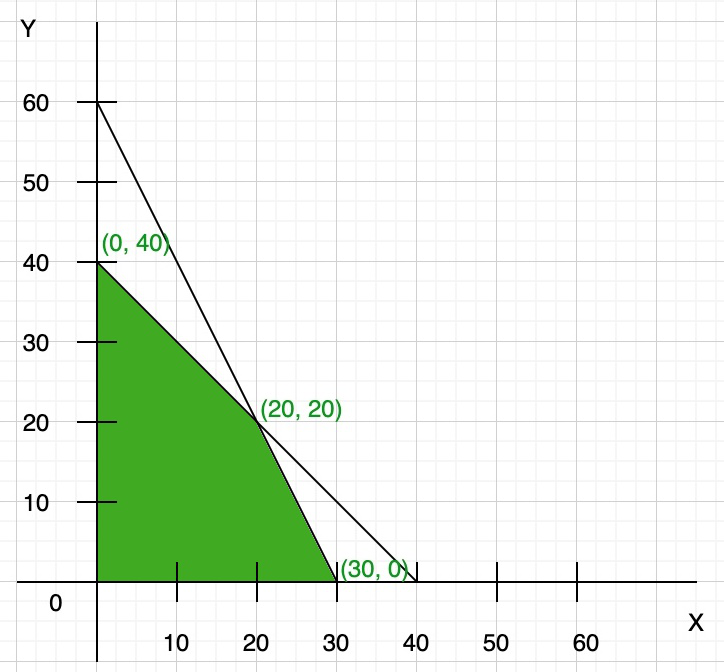
Here both the constraints are less than or equal to, so they satisfy the below region (towards origin). You can find the vertex of feasible region by graph, or you can calculate using the given constraints:
x + y = 40 …(i)
2x + y = 60 …(ii)
Now multiply eq(i) by 2 and then subtract both eq(i) and (ii), we get
y = 20
Now put the value of y in any of the equations, we get
x = 20
So the third point of the feasible region is (20, 20)
Step 3: To find the maximum value of Z = 8x + y. Compare each intersection point of the graph to find the maximum value
| Points | Z = 8x + y |
|---|---|
| (0, 0) | 0 |
| (0, 40) | 40 |
| (20, 20) | 180 |
| (30, 0) | 240 |
So the maximum value of Z = 240 at point x = 30, y = 0.
Example 2: One kind of cake requires 200 g of flour and 25g of fat, and another kind of cake requires 100 g of flour and 50 g of fat Find the maximum number of cakes that can be made from 5 kg of flour and 1 kg of fat assuming that there is no shortage of the other ingredients, used in making the cakes.
Solution:
Step 1: Create a table like this for easy understanding (not necessary).
| Flour(g) | Fat(g) | |
|---|---|---|
| Cake of first kind (x) | 200 | 25 |
| Cake of second kind (y) | 100 | 50 |
| Availability | 5000 | 1000 |
Step 2: Create linear equation using inequality
- 200x + 100y ≤ 5000 or 2x + y ≤ 50
- 25x + 50y ≤ 1000 or x + 2y ≤ 40
- Also, x > 0 and y > 0
Step 3: Create a graph using the inequality (remember only to take positive x and y-axis)
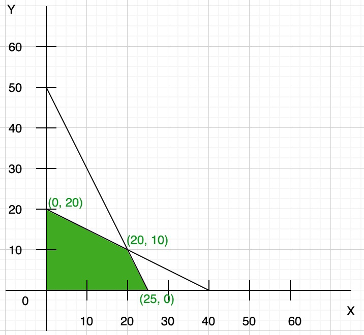
Step 4: To find the maximum number of cakes (Z) = x + y. Compare each intersection point of the graph to find the maximum number of cakes that can be baked.
| x | y | Z = (x+y) |
|---|---|---|
| 0 | 20 | 20 |
| 20 | 10 | 30 |
| 25 | 0 | 25 |
Clearly, Z is maximum at co-ordinate (20, 10). So the maximum number of cakes that can be baked is Z = 20 + 10 = 30.
Iso-Cost Methods
The term iso-cost or iso-profit method provides the combination of points that produces the same cost/profit as any other combination on the same line. This is done by plotting lines parallel to the slope of the equation.
To solve the problem using Iso-cost method you need to follow the following steps:
Step 1: Create mathematical formulation from the given problem. If not given.
Step 2: Now plot the graph using the given constraints and find the feasible region.
Step 3: Now find the coordinates of the feasible region that we get from step 2.
Step 4: Find the convenient value of Z(objective function) and draw the line of this objective function.
Step 5: If the objective function is maximum type then draw a line which is parallel to the objective function line and this line is farthest from the origin and only has one common point to the feasible region. Or if the objective function is minimum type then draw a line which is parallel to the objective function line and this line is nearest from the origin and has at least one common point to the feasible region.
Step 6: Now get the coordinates of the common point that we find in step 5. Now, this point is used to find the optimal solution and the value of the objective function.
Read More,
Solved Examples of Graphical Solution of LPP
Example 1: Solve the given linear programming problems graphically:
Maximize: Z = 50x + 15y
Constraints are,
- 5x + y ≤ 100
- x + y ≤ 50
- x ≥ 0, y ≥ 0
Solution:
Given,
- 5x + y ≤ 100
- x + y ≤ 50
- x ≥ 0, y ≥ 0
Step 1: Finding points
We can also write as
5x + y = 100….(i)
x + y = 50….(ii)
Now we find the points
so we take eq(i), now in this equation
When x = 0, y = 100
When y = 0, x = 20
So, points are (0, 100) and (20, 0)
Similarly, in eq(ii)
When x = 0, y = 50
When y = 0, x = 50
So, points are (0, 50) and (50, 0)
Step 2: Now plot these points in the graph and find the feasible region.
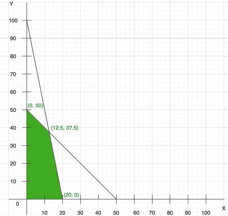
Step 3: Now we find the convenient value of Z(objective function)
So, to find the convenient value of Z, we have to take the lcm of coefficient of 50x + 15y, i.e., 150. So, the value of Z is the multiple of 150, i.e., 300. Hence,
50x + 15y = 300
Now we find the points
Put x = 0, y = 20
Put y = 0, x = 6
draw the line of this objective function on the graph:
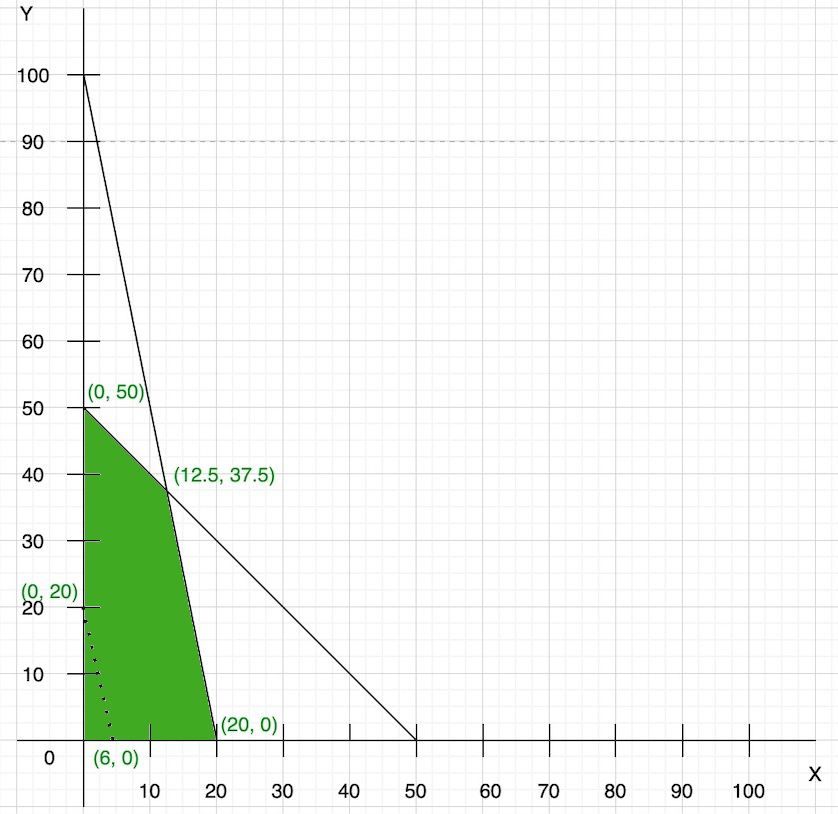
Step 4: As we know that the objective function is maximum type then we draw a line which is parallel to the objective function line and farthest from the origin and only has one common point to the feasible region.
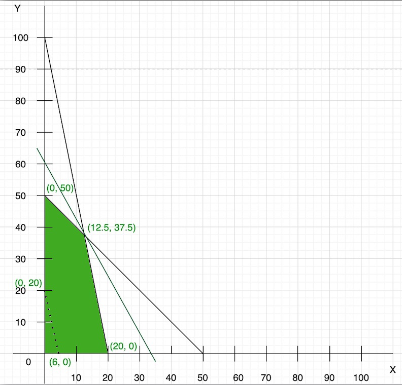
Step 5: We have a common point that is (12.5, 37.5) with the feasible region. So, now we find the optimal solution of the objective function:
Z = 50x + 15y
Z = 50(12.5) + 15(37.5)
Z = 625 + 562.5
Z = 1187
Thus, maximum value of Z with given constraint is, 1187


Comments
Post a Comment