Equations of first order of partial differential equation

Equations of first order[edit]

Linear and nonlinear equations[edit]

Linear equations[edit]

A PDE is called linear if it is linear in the unknown and its derivatives. For example, for a function $u$ of $x$ and $y$ , a second order linear PDE is of the form

a_{1}(x,y)u_{xx}+a_{2}(x,y)u_{xy}+a_{3}(x,y)u_{yx}+a_{4}(x,y)u_{yy}+a_{5}(x,y)u_{x}+a_{6}(x,y)u_{y}+a_{7}(x,y)u=f(x,y)

where

a i

and

f

are functions of the independent variables only. (Often the mixed-partial derivatives

u xy

and

u yx

will be equated, but this is not required for the discussion of linearity.) If the

a i

are constants (independent of

x

and

y

) then the PDE is called linear with constant coefficients. If

f

is zero everywhere then the linear PDE is homogeneous, otherwise it is inhomogeneous. (This is separate from asymptotic homogenization, which studies the effects of high-frequency oscillations in the coefficients upon solutions to PDEs.)

Nonlinear equations[edit]

Three main types of nonlinear PDEs are semilinear PDEs, quasilinear PDEs, and fully nonlinear PDEs.

Nearest to linear PDEs are semilinear PDEs, where only the highest order derivatives appear as linear terms, with coefficients that are functions of the independent variables. The lower order derivatives and the unknown function may appear arbitrarily. For example, a general second order semilinear PDE in two variables is

a_{1}(x,y)u_{xx}+a_{2}(x,y)u_{xy}+a_{3}(x,y)u_{yx}+a_{4}(x,y)u_{yy}+f(u_{x},u_{y},u,x,y)=0

In a quasilinear PDE the highest order derivatives likewise appear only as linear terms, but with coefficients possibly functions of the unknown and lower-order derivatives:

a_{1}(u_{x},u_{y},u,x,y)u_{xx}+a_{2}(u_{x},u_{y},u,x,y)u_{xy}+a_{3}(u_{x},u_{y},u,x,y)u_{yx}+a_{4}(u_{x},u_{y},u,x,y)u_{yy}+f(u_{x},u_{y},u,x,y)=0

Many of the fundamental PDEs in physics are quasilinear, such as the Einstein equations of general relativity and the Navier–Stokes equations describing fluid motion.

A PDE without any linearity properties is called fully nonlinear, and possesses nonlinearities on one or more of the highest-order derivatives. An example is the Monge–Ampère equation, which arises in differential geometry.^[3]

Linear equations of second order[edit]

Elliptic, parabolic, and hyperbolic partial differential equations of order two have been widely studied since the beginning of the twentieth century. However, there are many other important types of PDE, including the Korteweg–de Vries equation. There are also hybrids such as the Euler–Tricomi equation, which vary from elliptic to hyperbolic for different regions of the domain. There are also important extensions of these basic types to higher-order PDE, but such knowledge is more specialized.

The elliptic/parabolic/hyperbolic classification provides a guide to appropriate initial and boundary conditions and to the smoothness of the solutions. Assuming $u xy = u yx$ , the general linear second-order PDE in two independent variables has the form

Au_{xx}+2Bu_{xy}+Cu_{yy}+\cdots {\mbox{(lower order terms)}}=0,

where the coefficients

A

B

C

... may depend upon

x

and

y

. If

A 2 + B 2 + C 2 > 0

over a region of the

xy

-plane, the PDE is second-order in that region. This form is analogous to the equation for a conic section:

Ax^{2}+2Bxy+Cy^{2}+\cdots =0.

More precisely, replacing $\partial x$ by $X$ , and likewise for other variables (formally this is done by a Fourier transform), converts a constant-coefficient PDE into a polynomial of the same degree, with the terms of the highest degree (a homogeneous polynomial, here a quadratic form) being most significant for the classification.

Just as one classifies conic sections and quadratic forms into parabolic, hyperbolic, and elliptic based on the discriminant $B 2 - 4 AC$ , the same can be done for a second-order PDE at a given point. However, the discriminant in a PDE is given by $B 2 - AC$ due to the convention of the $xy$ term being $2 B$ rather than $B$ ; formally, the discriminant (of the associated quadratic form) is $(2 B) 2 - 4 AC = 4(B 2 - AC)$ , with the factor of 4 dropped for simplicity.

$B 2 - AC < 0$ (elliptic partial differential equation): Solutions of elliptic PDEs are as smooth as the coefficients allow, within the interior of the region where the equation and solutions are defined. For example, solutions of Laplace's equation are analytic within the domain where they are defined, but solutions may assume boundary values that are not smooth. The motion of a fluid at subsonic speeds can be approximated with elliptic PDEs, and the Euler–Tricomi equation is elliptic where $x < 0$ .
$B 2 - AC = 0$ (parabolic partial differential equation): Equations that are parabolic at every point can be transformed into a form analogous to the heat equation by a change of independent variables. Solutions smooth out as the transformed time variable increases. The Euler–Tricomi equation has parabolic type on the line where $x = 0$ .
$B 2 - AC > 0$ (hyperbolic partial differential equation): hyperbolic equations retain any discontinuities of functions or derivatives in the initial data. An example is the wave equation. The motion of a fluid at supersonic speeds can be approximated with hyperbolic PDEs, and the Euler–Tricomi equation is hyperbolic where $x > 0$ .

If there are $n$ independent variables $x 1, x 2, \dots, x n$ , a general linear partial differential equation of second order has the form

Lu=\sum _{i=1}^{n}\sum _{j=1}^{n}a_{i,j}{\frac {\partial ^{2}u}{\partial x_{i}\partial x_{j}}}\quad +{\text{lower-order terms}}=0.

The classification depends upon the signature of the eigenvalues of the coefficient matrix $a i, j$ .

Elliptic: the eigenvalues are all positive or all negative.
Parabolic: the eigenvalues are all positive or all negative, except one that is zero.
Hyperbolic: there is only one negative eigenvalue and all the rest are positive, or there is only one positive eigenvalue and all the rest are negative.
Ultrahyperbolic: there is more than one positive eigenvalue and more than one negative eigenvalue, and there are no zero eigenvalues.^[4]

The theory of elliptic, parabolic, and hyperbolic equations have been studied for centuries, largely centered around or based upon the standard examples of the Laplace equation, the heat equation, and the wave equation.

Systems of first-order equations and characteristic surfaces[edit]

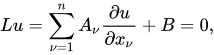
The classification of partial differential equations can be extended to systems of first-order equations, where the unknown $u$ is now a vector with $m$ components, and the coefficient matrices $A ν$ are $m$ by $m$ matrices for $ν = 1, 2, \dots, n$ . The partial differential equation takes the form

Lu=\sum _{\nu =1}^{n}A_{\nu }{\frac {\partial u}{\partial x_{\nu }}}+B=0,

where the coefficient matrices

A ν

and the vector

B

may depend upon

x

and

u

. If a hypersurface

S

is given in the implicit form

\varphi (x_{1},x_{2},\ldots ,x_{n})=0,

where

φ

has a non-zero gradient, then

S

is a characteristic surface for the operator

L

at a given point if the characteristic form vanishes:

Q\left({\frac {\partial \varphi }{\partial x_{1}}},\ldots ,{\frac {\partial \varphi }{\partial x_{n}}}\right)=\det \left[\sum _{\nu =1}^{n}A_{\nu }{\frac {\partial \varphi }{\partial x_{\nu }}}\right]=0.

The geometric interpretation of this condition is as follows: if data for $u$ are prescribed on the surface $S$ , then it may be possible to determine the normal derivative of $u$ on $S$ from the differential equation. If the data on $S$ and the differential equation determine the normal derivative of $u$ on $S$ , then $S$ is non-characteristic. If the data on $S$ and the differential equation do not determine the normal derivative of $u$ on $S$ , then the surface is characteristic, and the differential equation restricts the data on $S$ : the differential equation is internal to $S$ .

A first-order system $Lu = 0$ is elliptic if no surface is characteristic for $L$ : the values of $u$ on $S$ and the differential equation always determine the normal derivative of $u$ on $S$ .
A first-order system is hyperbolic at a point if there is a spacelike surface $S$ with normal $ξ$ at that point. This means that, given any non-trivial vector $η$ orthogonal to $ξ$ , and a scalar multiplier $λ$ , the equation $Q (λξ + η) = 0$ has $m$ real roots $λ 1, λ 2, \dots, λ m$ . The system is strictly hyperbolic if these roots are always distinct. The geometrical interpretation of this condition is as follows: the characteristic form $Q (ζ) = 0$ defines a cone (the normal cone) with homogeneous coordinates ζ. In the hyperbolic case, this cone has $m$ sheets, and the axis $ζ = λξ$ runs inside these sheets: it does not intersect any of them. But when displaced from the origin by η, this axis intersects every sheet. In the elliptic case, the normal cone has no real sheets.

Analytical solutions[edit]

Separation of variables[edit]

Linear PDEs can be reduced to systems of ordinary differential equations by the important technique of separation of variables. This technique rests on a characteristic of solutions to differential equations: if one can find any solution that solves the equation and satisfies the boundary conditions, then it is the solution (this also applies to ODEs). We assume as an ansatz that the dependence of a solution on the parameters space and time can be written as a product of terms that each depend on a single parameter, and then see if this can be made to solve the problem.^[5]

In the method of separation of variables, one reduces a PDE to a PDE in fewer variables, which is an ordinary differential equation if in one variable – these are in turn easier to solve.

This is possible for simple PDEs, which are called separable partial differential equations, and the domain is generally a rectangle (a product of intervals). Separable PDEs correspond to diagonal matrices – thinking of "the value for fixed $x$ " as a coordinate, each coordinate can be understood separately.

This generalizes to the method of characteristics, and is also used in integral transforms.

Method of characteristics[edit]

In special cases, one can find characteristic curves on which the equation reduces to an ODE – changing coordinates in the domain to straighten these curves allows separation of variables, and is called the method of characteristics.

More generally, one may find characteristic surfaces. For a second order partial differential equation solution, see the Charpit method.

Integral transform[edit]

An integral transform may transform the PDE to a simpler one, in particular, a separable PDE. This corresponds to diagonalizing an operator.

An important example of this is Fourier analysis, which diagonalizes the heat equation using the eigenbasis of sinusoidal waves.

If the domain is finite or periodic, an infinite sum of solutions such as a Fourier series is appropriate, but an integral of solutions such as a Fourier integral is generally required for infinite domains. The solution for a point source for the heat equation given above is an example of the use of a Fourier integral.

Change of variables[edit]

Often a PDE can be reduced to a simpler form with a known solution by a suitable change of variables. For example, the Black–Scholes equation

{\frac {\partial V}{\partial t}}+{\tfrac {1}{2}}\sigma ^{2}S^{2}{\frac {\partial ^{2}V}{\partial S^{2}}}+rS{\frac {\partial V}{\partial S}}-rV=0

is reducible to the heat equation

{\frac {\partial u}{\partial \tau }}={\frac {\partial ^{2}u}{\partial x^{2}}}

by the change of variables^[6]

{\begin{aligned}V(S,t)&=v(x,\tau ),\\[5px]x&=\ln \left(S\right),\\[5px]\tau &={\tfrac {1}{2}}\sigma ^{2}(T-t),\\[5px]v(x,\tau )&=e^{-\alpha x-\beta \tau }u(x,\tau ).\end{aligned}}

Fundamental solution[edit]

Inhomogeneous equations^{[clarification needed]} can often be solved (for constant coefficient PDEs, always be solved) by finding the fundamental solution (the solution for a point source), then taking the convolution with the boundary conditions to get the solution.

This is analogous in signal processing to understanding a filter by its impulse response.

Superposition principle[edit]

The superposition principle applies to any linear system, including linear systems of PDEs. A common visualization of this concept is the interaction of two waves in phase being combined to result in a greater amplitude, for example $sin x + sin x = 2 sin x$ . The same principle can be observed in PDEs where the solutions may be real or complex and additive. If $u 1$ and $u 2$ are solutions of linear PDE in some function space $R$ , then $u = c 1 u 1 + c 2 u 2$ with any constants $c 1$ and $c 2$ are also a solution of that PDE in the same function space.

Methods for non-linear equations[edit]

There are no generally applicable methods to solve nonlinear PDEs. Still, existence and uniqueness results (such as the Cauchy–Kowalevski theorem) are often possible, as are proofs of important qualitative and quantitative properties of solutions (getting these results is a major part of analysis). Computational solution to the nonlinear PDEs, the split-step method, exist for specific equations like nonlinear Schrödinger equation.

Nevertheless, some techniques can be used for several types of equations. The $h$ -principle is the most powerful method to solve underdetermined equations. The Riquier–Janet theory is an effective method for obtaining information about many analytic overdetermined systems.

The method of characteristics can be used in some very special cases to solve nonlinear partial differential equations.^[7]

In some cases, a PDE can be solved via perturbation analysis in which the solution is considered to be a correction to an equation with a known solution. Alternatives are numerical analysis techniques from simple finite difference schemes to the more mature multigrid and finite element methods. Many interesting problems in science and engineering are solved in this way using computers, sometimes high performance supercomputers.

Search This Blog

Dr. Balamurugan